Mortgage Pipeline Forecasting: A Practitioner’s Playbook

Mortgage pipeline forecasting estimates the share of locked loans in a lender’s pipeline that will actually fund, then uses that estimate to size hedge coverage. The core metric is pull-through: funded loan volume divided by locked loan volume within a given observation window, as MCT’s pull-through primer lays out. The recommendation for anyone running a secondary marketing desk in 2026 is straightforward.
- Build loan-level, stage-adjusted expected funded volume, not a single blended pull-through number for the whole pipeline.
- Layer in a market beta adjustment so hedge coverage moves with rate direction instead of lagging it.
- Treat forecast accuracy as a margin protection tool, not a reporting exercise. A pipeline that’s over-hedged bleeds carry cost every day; one that’s under-hedged exposes the lender to price risk on every basis point move.
Key Takeaways
Accurate mortgage pipeline forecasting combines loan-level, stage-adjusted pull-through estimates with a market beta adjustment to set hedge coverage that tracks actual rate risk.
| Point | Details |
|---|---|
| Define pull-through precisely | Calculate funded volume divided by locked volume within a set window, by stage, not as one blended pipeline figure. |
| Model at the loan level | Score FICO, channel, loan officer, and pricing context individually, then sum into expected funded volume. |
| Adjust for market beta | Regress historical pull-through deviation against rate moves to size hedges dynamically rather than statically. |
| Govern with a fixed cadence | Run daily drift checks, weekly hedge reviews, and quarterly stress tests against multiple rate regimes. |
| Automate borrower and pipeline signals | Loan Officer AI centralizes stage tracking, refi/HELOC detection, and automated follow-up to reduce fallout that pure rate models miss. |
Table of Contents
- Why Mortgage Pipeline Forecasting Matters for Hedging and Margin
- How Should You Structure Pipeline Stages for Forecasting?
- What Loan-Level Data Actually Improves Pipeline Forecasts?
- What Daily Signals Should Feed a Live Pipeline Forecast?
- How Do You Calculate Market Beta for Pull-Through Forecasting?
- How Do You Calculate Pipeline-Level Pull-Through Step by Step?
- Which Forecasting Model Should You Use: Logistic Regression or Machine Learning?
- What Data and Tools Do You Need for Live Forecasting?
- How Should You Govern and Monitor Pipeline Forecasts?
- How Do Economic Indicators and Housing Trends Affect Pipeline Forecasts?
- How Does Pipeline Forecasting Fit Into Enterprise Risk Management?
- What Are the Biggest Pitfalls in Mortgage Pipeline Forecasting?
- How Should You Stress Test Pipeline Forecasts?
- What Role Does Technology Play in Forecast Accuracy?
- Why Integrated Borrower Signals Change What Forecasting Can Actually Do
- How Loan Officer AI Supports Pipeline Forecasting in Practice
- Frequently Asked Questions
- Sources
Why Mortgage Pipeline Forecasting Matters for Hedging and Margin
Get the forecast wrong in either direction and it costs money. Over-hedge the pipeline and you’re carrying excess TBA or forward commitments that generate negative carry and transaction costs with no offsetting risk reduction. Under-hedge it and a sudden rate move against an unhedged slice of locked loans erodes margin loan by loan, often invisibly until month-end reconciliation.
Statistic Callout: A random forest model built on a large U.S. lender dataset predicted loan fallout with roughly 74% accuracy, a meaningful jump over cruder heuristic approaches that treat every loan in a stage identically.
Three KPIs deserve a permanent spot on the secondary desk’s dashboard:
- Pull-through volatility, measured week over week against a rolling baseline.
- Hedge tracking error, the gap between hedge notional and actual funded notional at settlement.
- Funded timing variance, since a loan that funds three weeks later than modeled still creates duration mismatch even if the volume estimate was correct.
How Should You Structure Pipeline Stages for Forecasting?
A forecast built on a single blended pull-through rate is a forecast built on sand. Loans in different stages carry wildly different fallout risk, and lumping them together hides the signal you actually need.
A workable stage taxonomy looks like this:
- Application — earliest stage, highest fallout risk, most sensitive to shopping and rate competition.
- Approval — underwriting conditions cleared, borrower commitment more established.
- Clear to close (CTC) — nearly all conditions satisfied, fallout risk drops sharply.
- Committed — rate locked with a defined expiration, borrower has skin in the game.
- Pre-fund — closing scheduled, fallout is now almost entirely operational (title issues, wire delays) rather than borrower choice.
Time-in-stage matters as much as the stage label itself. A loan that’s spent six days in CTC behaves differently than one that just arrived there, and operational levers like lock-desk policy that push commitment deeper into the process measurably raise pull-through certainty. The longer a loan sits deep in the pipeline without falling out, the less sensitive its outcome becomes to a rate move elsewhere in the market.
Pro Tip:Track median time-in-stage separately for each loan officer or branch. A branch with unusually fast CTC times often has looser underwriting discipline, and that shows up later as elevated fallout, not as a forecasting win.
What Loan-Level Data Actually Improves Pipeline Forecasts?
Aggregate pull-through heuristics, applying one flat percentage to the whole pipeline, miss the variance that actually drives hedging error. Loan-level modeling fixes this by scoring each loan individually and summing the results into an expected funded volume figure.
The features that carry real predictive weight include:
- Loan characteristics: loan amount, product type, rate lock expiration, current pipeline stage.
- Borrower attributes: FICO score, debt-to-income ratio, purpose (purchase versus refinance).
- Pricing context: note rate relative to current market rate, since a borrower with a rate well below market has little incentive to walk.
- Origination channel: retail, wholesale, or correspondent, each with distinct historical fallout patterns.
- Loan officer and branch identity, which the MDPI fallout study identified, alongside loan stage and FICO, as one of the strongest predictors of outcome.
To convert this into expected funded volume, multiply each loan’s individual pull-through probability by its locked amount, then sum across the pipeline. Compare that to the naive approach: apply a recent blended pull-through rate to every loan regardless of stage or channel. The naive method might land close on a stable month and miss badly by several percentage points the moment channel mix shifts or a batch of loans clusters near lock expiration, exactly when hedge sizing errors hurt most.
What Daily Signals Should Feed a Live Pipeline Forecast?
A forecast refreshed once a month is a forecast that’s already wrong by the time anyone acts on it. Daily and weekly signals need different handling because they move at different speeds and carry different weight.
Priority daily signals worth pulling every morning:
- Locks expiring within the next five business days, since these convert or fall out fastest.
- New approvals and conditional approvals clearing underwriting.
- Appraisal and underwriting flags that indicate a stalled or at-risk file.
Weekly and monthly signals that shift the baseline rather than the day’s number:
- Pricing and rate moves across the note-rate distribution of the pipeline.
- Implied volatility trends that affect how borrowers respond to rate changes.
- Channel-level trend shifts, such as a correspondent partner’s volume ramping or slowing.
Pro Tip:Weight daily signals with a short time-decay window, roughly five to ten business days, so a stale underwriting flag doesn’t keep dragging a loan’s score down after the issue is resolved.
How Do You Calculate Market Beta for Pull-Through Forecasting?
Pull-through isn’t static. It moves with rates, and the relationship runs in a specific direction: when rates fall, existing locks become more valuable but a smaller share ultimately funds because borrowers shop for something better; when rates rise, locks are worth less but a larger share tends to fund because refinancing elsewhere loses its appeal, a pattern MCT’s research documents clearly. Market beta quantifies that sensitivity so the hedge desk can adjust coverage before the move shows up in funded volume.
The calculation flow runs in three stages:
- Run a regression of historical market rate moves (basis points) against realized pull-through deviations from baseline, using logistic regression, random forest, or XGBoost depending on how much nonlinearity the data shows.
- Apply the resulting slope to the current market move to adjust each loan’s stage-baseline pull-through up or down.
- Multiply the adjusted pull-through by locked amount across the pipeline to get expected funded notional, then size TBA or forward commitments to match that notional.
The biggest hedging failures rarely come from a bad model. They come from a good model whose output nobody adjusted for a market move that happened between forecast runs.
Three pitfalls recur across secondary desks: basis risk between TBA coupons and the actual loans in the pipeline, negative convexity that makes mortgage-backed hedges lose value faster than they gain it, and rebalancing costs that pile up when a desk chases every small pull-through revision instead of setting a threshold for action. Milliman’s overview of pipeline hedging covers the duration and convexity mechanics in more depth.
How Do You Calculate Pipeline-Level Pull-Through Step by Step?
The full recipe, applied to a rolling data set, breaks into seven steps:
- Extract locked and funded loan records for a defined historical window, typically 12 to 24 months.
- Compute baseline pull-through by stage using only that historical data, isolated from any market movement.
- Calculate the market experience (rate move at lock versus rate at outcome) for each historical loan.
- Regress pull-through deviation against that market experience to get the beta coefficient.
- Recompute a zero-market baseline pull-through rate for each stage, stripping out the historical rate effect.
- Apply today’s actual market move through the beta coefficient to adjust the baseline for the current pipeline.
- Weight-average the adjusted, loan-level pull-through by locked balance to get a single pipeline-level forecast.
Watch for two common data issues: locks that were modified or relocked (they inflate apparent fallout if not tracked as the same loan) and funded loans mismatched to the wrong lock date. The resulting percentage feeds directly into hedge-sizing automation, which is where the calculation earns its keep rather than sitting in a spreadsheet nobody rechecks.
Which Forecasting Model Should You Use: Logistic Regression or Machine Learning?
Logistic regression remains a solid starting point when the pipeline is small, the relationships between features are mostly linear, and the team needs a model that’s easy to explain to a risk committee in one sentence. It struggles once channel mix, loan officer effects, and rate sensitivity start interacting in nonlinear ways, which is common in any pipeline spanning retail, wholesale, and correspondent originations.
Tree-based methods close that gap. The MDPI study on fallout prediction found random forest outperformed logistic regression and other alternatives on a large lender dataset, and XGBoost tends to perform comparably while training faster on larger feature sets. The trade-off is interpretability, which is where SHAP (Shapley Additive Explanations) earns its place in the workflow: it decomposes each prediction into the contribution of individual features, turning a black-box fallout score into something a hedge desk can act on, such as “this batch of loans is scoring low on pull-through mainly because of originating channel, not FICO.”
Statistic Callout: SHAP analysis in the same study identified loan stage, originating division, and FICO score as the three leading predictors of fallout, which lines up with what most secondary desks already suspect but rarely quantify.
A validation checklist worth running quarterly:
- ROC/AUC to measure overall discrimination between funded and fallout loans.
- Calibration checks, confirming that a loan scored at 80% pull-through actually funds around 80% of the time.
- F1 score where fallout is the minority class and false negatives carry real cost.
- Stability testing across at least two different rate regimes, since a model trained entirely in a falling-rate environment often mispredicts badly once rates reverse.
What Data and Tools Do You Need for Live Forecasting?
Live pipeline forecasting depends on a handful of data sources arriving on a predictable schedule. The loan origination system (LOS) supplies stage and status data. The lock desk or pricing engine supplies rate lock terms and expiration dates. Underwriting and appraisal systems flag conditions that stall a file. Channel attribution data, retail versus wholesale versus correspondent, ties outcomes back to origination source.

Integration is where most forecasting projects stall out. Latency matters: a forecast running on data that’s a day and a half old misses locks expiring that afternoon. Schema consistency matters just as much, since a stage label that means one thing in the LOS and another in a legacy reporting extract will quietly corrupt the model’s training data. Automated quality checks, flagging duplicate lock IDs or missing funding dates, catch problems before they reach the hedge desk.
Beyond raw data, three components turn a forecast into an operational tool rather than a report: a dashboard showing pipeline-level pull-through and hedge tracking error in one view, alerting on loans nearing lock expiration or stalled in underwriting, and an automated hook that proposes rebalancing trades rather than waiting for someone to notice drift. A platform built around pipeline management that centralizes these signals removes a step most teams currently do by hand in a spreadsheet.
How Should You Govern and Monitor Pipeline Forecasts?
Forecasts decay without ownership. A model owner should be accountable for the pull-through model itself, with a designated secondary reviewer who can validate outputs when the owner is unavailable, and a QA function that checks incoming data before it reaches production.
Monitoring cadence matters more than model sophistication. A workable rhythm:
- Daily automated drift detection comparing predicted versus actual fallout on loans that resolved that day.
- Weekly hedge review comparing hedge notional against expected funded notional, flagging tracking error beyond a set threshold.
- Monthly post-trade reconciliation against actual settlement to catch systematic bias building up slowly.
- Quarterly stress-test runs against historical rate shock scenarios to confirm the model still behaves reasonably under conditions it hasn’t recently seen.
Pro Tip:Set a conservative fallback pull-through assumption, lower than the model’s typical output, that automatically triggers if daily drift detection flags an anomaly. A model that’s temporarily wrong is far less dangerous than a hedge desk that keeps trusting it anyway.
How Do Economic Indicators and Housing Trends Affect Pipeline Forecasts?
Rate direction is the dominant economic input, but it’s not the only one that moves pull-through in a given quarter. Mortgage applications respond to the 10-year Treasury yield with a lag of days, not months, since lenders reprice almost immediately while borrower behavior takes longer to shift. A pipeline built during a stretch of falling rates will show elevated refinance fallout risk months later if rates stabilize, because the borrowers most likely to shop for a better deal are exactly the ones with locks still open.
Housing inventory and home price trends matter more for purchase-heavy pipelines than refinance-heavy ones. When inventory is tight and bidding is competitive, purchase transactions that reach a signed contract tend to close at high rates because buyers have already cleared financing hurdles before locking. When inventory loosens and price growth slows, purchase pull-through can soften as buyers walk away from deals or renegotiate financing terms mid-transaction.
Employment data and consumer sentiment feed into fallout risk indirectly, through debt-to-income recalculations and appraisal disputes rather than through the lock decision itself. A borrower who loses income between application and closing generates an underwriting-stage fallout event that a purely rate-driven model won’t anticipate.
The practical implication for forecasting teams: don’t build a single model that assumes refinance and purchase loans respond to the same macro inputs the same way. Segment the pipeline by loan purpose before applying market beta adjustments, since a 25 basis point rate increase might raise refinance pull-through while barely moving purchase pull-through at all. Teams that skip this segmentation tend to overcorrect one segment while leaving the other under-hedged.
How Does Pipeline Forecasting Fit Into Enterprise Risk Management?
Pipeline forecasting shouldn’t live in a silo on the secondary marketing desk. The hedge positions it drives interact directly with the lender’s balance sheet, liquidity planning, and interest rate risk framework, which means the forecast needs to speak the same language as the enterprise risk function.
The clearest integration point is interest rate risk. A pipeline hedge desk manages short-duration exposure measured in weeks, while the asset-liability committee manages longer-horizon exposure across the loan portfolio and any retained servicing rights. Both are exposed to the same underlying rate moves, so a lender that treats pipeline hedging as fully separate from enterprise interest rate risk reporting ends up with a fragmented view of total exposure at any given moment.
Liquidity planning is the second point of overlap. Expected funded volume from the pipeline forecast feeds directly into warehouse line utilization projections. A forecast that consistently overestimates funded volume ties up warehouse capacity that could be deployed elsewhere; one that underestimates it risks a capacity crunch during a funding surge.
Capital and credit risk functions care about pipeline forecasting too, though less obviously. Fallout patterns tied to FICO or debt-to-income shifts can be an early signal of broader credit quality drift in the origination channel, information that’s valuable to the credit risk team well before it shows up in delinquency data months later.
Governance frameworks that treat pipeline forecasting as a stand-alone secondary marketing function, reviewed only by the trading desk, miss these connections. A more resilient structure routes pipeline forecast outputs, tracking error, and stress-test results into the same risk committee that reviews interest rate risk and liquidity, even if the day-to-day hedging decisions stay with the secondary team.
What Are the Biggest Pitfalls in Mortgage Pipeline Forecasting?
The most common failure mode is treating pull-through as a single number instead of a distribution that shifts by stage, channel, and market condition. A lender that applies last quarter’s blended rate to this quarter’s pipeline is essentially forecasting with a rearview mirror, and it works fine right up until the market moves.
Data quality problems cause the second-most common failure. Relocked loans that get counted as new locks inflate apparent fallout. Funding dates recorded against the wrong lock create phantom timing variance. Channel attribution that’s inconsistently tagged between the LOS and the accounting system quietly breaks channel-level model segments without anyone noticing until the forecast starts missing by a consistent margin in one direction.
Overfitting to a single rate regime is a subtler trap. A model trained mostly on a two-year stretch of falling rates learns patterns that don’t hold once rates reverse, and because the model’s historical accuracy metrics look strong, teams tend to trust it past the point where it should be recalibrated. Stability testing across regimes, mentioned earlier as part of the validation checklist, exists specifically to catch this before it costs real hedging dollars.
Organizational pitfalls matter as much as technical ones. Forecasts that live only with the secondary desk, with no cross-check from operations or risk management, tend to drift without anyone questioning the assumptions baked in months earlier. And teams that chase every small forecast revision with a hedge rebalance rack up transaction costs that erase the benefit of the more precise forecast in the first place.
The mitigation across all of these is the same: segment the pipeline, validate the model against fresh data on a fixed cadence, and set a threshold for when a forecast change actually warrants a trade rather than reacting to every revision.
How Should You Stress Test Pipeline Forecasts?
Scenario analysis answers a question point forecasts can’t: what happens to the pipeline and its hedge if the market moves further, or faster, than the model’s training data ever saw. A pull-through model calibrated on the past two years is only as good as the range of conditions in that window, and rate moves have a habit of exceeding recent ranges precisely when it matters most.
A useful stress-testing framework runs at least three scenario types. Parallel rate shocks, moving the entire yield curve up or down by a fixed amount, test whether the market beta adjustment holds at the extremes rather than just near the center of its calibration range. Channel-mix shocks, simulating a sudden shift toward correspondent or wholesale volume, test whether the model’s channel-level assumptions break down under a mix the historical data underrepresents. Operational shock scenarios, like a spike in appraisal delays or underwriting backlogs, test the model’s sensitivity to fallout drivers that have nothing to do with rates at all.
Validation against these scenarios should compare not just the point forecast but the confidence interval around it. A model that produces a tight, confident pull-through estimate under a stress scenario it’s never been tested against is a red flag, not a reassurance. Wider uncertainty under stress is the honest answer, and a hedging strategy that assumes otherwise is the one most likely to be caught under-covered when a shock actually hits.
The output of stress testing should feed directly into the fallback controls covered earlier in governance: a conservative pull-through cap that activates automatically, and a manual override trigger available to the model owner, both calibrated using the same stress scenarios rather than a number picked out of caution alone. Running these tests quarterly, alongside the validation checklist, keeps the model honest about the range of conditions it can actually be trusted in.
What Role Does Technology Play in Forecast Accuracy?
Model quality only goes as far as the data feeding it, and that’s where technology platforms earn their place in the forecasting workflow. A forecast that depends on someone manually pulling stage data from the LOS once a week is a forecast that’s structurally incapable of catching a fast-moving market or a batch of locks approaching expiration mid-week.
Automation closes that gap in three specific ways. It shortens the data latency between an event happening (a loan clearing underwriting, a lock expiring) and that event reaching the model, which matters because a robust forecasting workflow depends on daily extraction and an overnight model refresh rather than a weekly manual pull. It reduces the manual error rate in stage and channel tagging, since automated data pipelines apply consistent rules where manual entry introduces drift. And it makes the forecast actionable rather than descriptive, since an automated dashboard that flags loans nearing lock expiration or stalled in underwriting gives the desk something to act on the same day, not a report to review next week.
The database mining layer deserves specific mention here. Tools that continuously score a lender’s existing loan database for refinance and equity opportunities generate a secondary forecasting input: pipeline volume that hasn’t locked yet but is statistically likely to within a defined window, which matters for capacity planning even before those loans enter the formal pull-through model. Partner data services, such as property and equity data integrations, add another layer by supplying current valuation context that sharpens borrower-level fallout scoring beyond what the LOS alone provides.
Why Integrated Borrower Signals Change What Forecasting Can Actually Do
Most fallout gets attributed to rates, but a large share traces back to something more mundane: a borrower who went quiet, missed a document request, or got a better offer nobody flagged in time. Real-time signals on borrower activity, tied directly into automated follow-up, catch that drift before it becomes a lost loan, which changes the pull-through math for the whole pipeline rather than just the loans a human happened to notice.

That’s the piece a stage-and-market model alone can’t see, and it’s why forecasting and borrower engagement belong in the same workflow, not separate systems reviewed on different schedules.
How Loan Officer AI Supports Pipeline Forecasting in Practice
Everything covered above, stage-based baselines, loan-level scoring, market beta adjustments, depends on data arriving clean, current, and connected to what’s actually happening with each borrower. That’s the operational gap most forecasting efforts hit first, not the modeling itself.
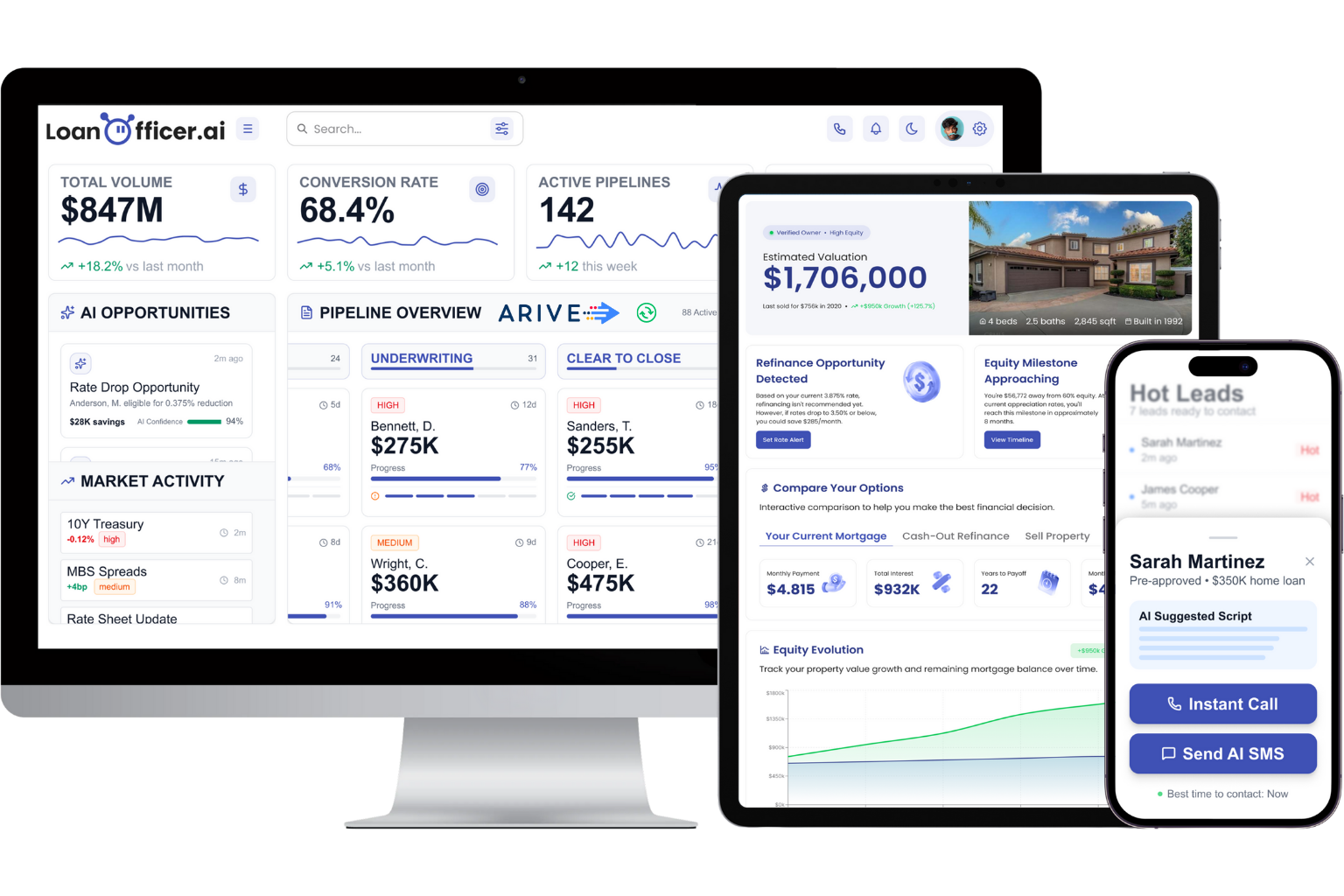
Loan Officer AI centralizes the signals a pipeline forecast actually needs: real-time pipeline management that tracks stage movement as it happens, automated detection of refinance and equity opportunities mining the existing database, and LOS integrations that keep stage and status data current instead of a day stale. Automated multi-channel follow-up addresses the borrower-drift fallout driver directly, catching the quiet-borrower risk that a market-beta model can’t see on its own.
If your forecasts are only as good as the data feeding them, start with the mortgage CRM built for this exact workflow and get a live look at how automated signals tighten pull-through accuracy before your next hedge review.
Frequently Asked Questions
What is a good pull-through rate for a mortgage pipeline? There’s no universal benchmark since pull-through varies by channel, loan purpose, and rate environment. What matters more than the absolute number is whether your forecast tracks the realized rate closely enough to keep hedge tracking error inside an acceptable range.
How often should pull-through forecasts be updated? Stage and underwriting data should refresh daily, with the pull-through model itself recalibrated at least monthly and stress-tested quarterly against different rate regimes.
What’s the difference between a mortgage pipeline and a pipeline hedge? The pipeline itself is the backlog of locked applications awaiting closing. The hedge is the separate position, typically TBAs, taken to protect the lender’s economics on that pipeline between lock and funding.
Why does explainability matter for fallout prediction models? SHAP and similar techniques let a hedge desk see which specific features, stage, channel, or FICO, are driving a fallout score, which builds the trust needed to act on model output instead of overriding it manually.
Can small mortgage teams use loan-level forecasting without a data science team? Yes, provided the underlying data (LOS stage, lock terms, borrower attributes) is centralized and clean. Platforms built around automated pipeline management handle much of the scoring and alerting that would otherwise require dedicated modeling staff.
Sources
- Pipeline Pull-through Rate Analysis Explained
- Explainable machine learning for fallout prediction in the mortgage pipeline (MDPI, 2024)
- Introduction to mortgage secondary pipeline hedging